As mentioned in the previous post, I want to start getting more information about the visual properties of artworks in the WCMA collection. The WCMA collection includes a set of thumbnails that I will be processing. Not every object in the collection has a thumbnail, but I will be able to learn more about the objects that do have thumbnails.
I will be using OpenCV to process the images. My code is available on Github; specifically, get_color_details.py.
One visual quality is color. My initial intuition is to get the “average” color of each thumbnail, but that may not be a very useful metric for pieces that are not monochromatic; a reply on this Stack Overflow post talks more in-depth about why it may be better to calculate the dominant colors in an image. We can use k-means clustering to get the k most representative colors for each thumbnail. This is essentially color quantization, or reducing the number of colors in an image. Taking the most representative color using this method would still be a little more helpful than taking the RGB vector composed of means of each color channel; the post gives an example of how this “average” ends up meaningless in relation to the original image. If the picture is monochrome, then the two values will be very similar, and if the picture isn’t monochrome, then the average doesn’t make much sense. OpenCV provides a tutorial on using k-means clustering for color quantization.
Another quality that may be helpful is how bright or dark an image is. We can measure this quality by looking at the luminance of the image, since luminance most closely corresponds to brightness, which is a subjective attribute of light1. There are many ways to calculate brightness, perceived brightness2, or luminance, and the difference not only between which measure to use but also how to calculate each measure definitely warrants further research. This Stack Overflow post on determining brightness of RGB color discusses these topics and provides some formulas to use, as well as a resource for figuring out what exactly to look up. For now, I will be letting OpenCV choose which formula to use by using it to convert the image to greyscale, and then calculating the mean pixel brightness from the greyscale image.
We can also use luminance to calculate the contrast of an image, since contrast is the difference in luminance between two objects. I will not be doing feature detection in these thumbnails (perhaps in the future), so I cannot compare the difference between the image feature and the background (Weber contrast). Instead, I will be calculating the Michelson contrast for each thumbnail.
C = (Lmax - Lmin) / (Lmax + Lmin)
This is not the best measure, as any image with both black and white present will have maximum contrast, regardless of the ratio of dark to light in the thumbnail. There are more sophisticated ways to measure contrast, and I may delve deeper into implementing these in the future.
Now that I have generated the mentioned attributes for each piece in the collection with a thumbnail, I can look at trends in these attributes for the collection as a whole. The code can be found at analyze_color_details.py. I used Seaborn to make the following plots.
For color, I want to see what the dominant colors of the collection are; by putting all the dominant colors of each piece into a single array, I can effectively treat the array as an image, and do another color quantization to get the top 10 colors of the collection. For future visualizations, it may also be fun to visualize the RGB distribution of the colors.
As shown above, it seems beige/brown are the most dominant colors in the collection!
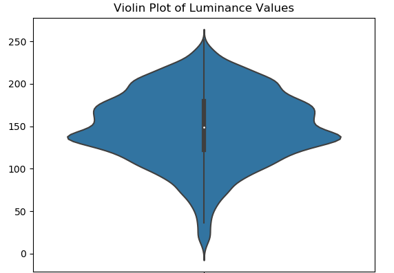
For luminance and contrast, which are single numbers, a histogram or box plot would tell me the most about the distribution of values in the collection.
The luminance values seem to be well-distributed; there are a decent amount of light and dark pieces, and the median luminance value is around 150. Luminance here is measured on a scale of 0 to 255, and scales linearly.
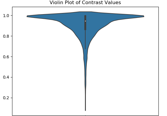
The distribution of contrast values is heavily skewed toward high-contrast, and this seems to be a result of the problem mentioned before: that any piece with a single white pixel and a single dark pixel will have a high contrast; this problem can be alleviated by using different contrast measures and also by doing feature detection on the thumbnails to try to get at a foreground/background contrast measure.